


Table of Contents
Introduction
As we know from our daily experience, air when it flows at a certain speed and hits our body we can feel it. Winds can be felt in the form of a breeze or can take great proportions like in the case of cyclones or tornadoes. While these forms clearly give us the experience that air does flow, what is not in direct experience is the fact that even when air is kept inside a tightly closed container, the individual atoms or molecules are still in a highly mobile state. Some simple experiments like keeping coloured gases inside transparent jars can easily help us comprehend this. This is called Maxwell-Boltzmann distribution. In this article, we'll look into the mechanism of how the movement of gases is related to their energies.
Origin of the idea
One might presume as per the kinetic theory, that all the gases are made up of identical particles that are always in motion. This was the concept that the generation brought up under Newtonian mechanics believed. It was widely accepted that since gas particles move about and encounter frequent collisions with each other, the velocity of these would average out. In the present day, it is a well-known fact that the motion of all the constituent atoms or molecules of gas however is not identical. In fact, there would be a highly unlikely scenario where two gaseous particles have identical properties in terms of their motions. Therefore, the speeds of the individual gaseous particles do vary widely, and while some of these move with great speed, some are more restful, but not totally still.
Distribution
This phenomenon of having particles with varying and random velocities brings us to something called “distribution”. Statistically, distribution means the probability of occurrence of a particular outcome from a given situation. In the present context, it means the possibility to classify the gaseous particles together on the basis of similarity in their speeds or velocities.
A point to remember and clearly understand in this context is that the “speed” of two particles can be equal but the “velocity” cannot be since it is impossible to have any two gaseous particles to have identical velocities because their motions are in random directions. This difference in velocities is crucial in the context of an effective number of collisions that these gaseous particles undergo with each other.
Kinetic energy
An important factor to be considered while studying the distribution of gaseous particles is temperature. The average kinetic energy is proportional to the temperature of the system. As the temperature varies, the average kinetic energy also varies which essentially is a reflection of the difference in the motion of the individual particles.
Relationship between speed and temperature
Considering these two aspects, one comes to a point where a question arises as to “How is the number of particles travelling at a certain speed relate to the temperature?” Newtonian mechanics of certainty did not have the scope for a concept of uncertainty. But the practical problem was that measuring the speeds of individual molecules.
But certainly, the concept of an average speed borne by all the molecules wasn’t the answer since such a situation goes against the concept of activation energy and the fact that only a certain amount of gases can react. The answer to this question was found in the 1800s by James Clerk Maxwell and Ludwig Boltzmann, working independently. In the present day, their work is known as the Maxwell-Boltzmann distribution.
Read more about Electron Configuration
Probability - the core of Boltzmann distribution
Motion of gaseous particles
Now coming to what exactly this relationship between temperature and the distribution of gaseous particles work out, we need to have a look at an example. Let’s assume a sealed container contains nitrogen gas (an ideal choice for such an experiment since it is unreactive; chemical reactions can significantly alter the observations). All the molecules therein are moving in random directions with different speeds. So any attempt to represent the speed of the molecules will have to include the number of molecules. We can plot the number of molecules (y-axis) vs the speed at which these move (x-axis). The x-axis can also be plotted as the kinetic energy.
Distribution of the particles
Maxwell postulated that the “distribution” or the ways in which the molecules moving with random speeds can be clubbed together to derive any meaningful information from their motions, would be similar to a “normal distribution”. A normal distribution refers to a continuous probability distribution. The mean, median, and the mode of the set of the available data in case of a normal distribution are equal. The data values are dispersed equally from the mean in case of a normal distribution.
In simple terms, it can help us in predicting the chance or probability of finding a value of a variable within a range. On one hand, this incorporation of statistical probability by Maxwell made it possible to understand why all the gaseous particles do not cross the activation energy while on the other, it explained the fact that it was not necessary to obtain an accurate measurement of individual velocities of all the particles. At the same time, the variation in the speeds of the individual molecules had to be taken into account. The wide variation in the kinetic energy of the molecules meant that the shape of the curve could not be symmetrical as in the case of regular normal distribution.
Nature of the Maxwell-Boltzmann curve
Since almost all the molecules vary in their speeds, it is obvious that the graph will be a smooth one without any sharp edges. Another important aspect regarding the shape of the graph is that it is not uniform. The curve is skewed to the left while a longer tail is present at the right end. This signifies that only a few gaseous molecules possess very high speeds. The left portion clearly indicates that the speed can never be negative and at the same time, it indicates that the number of molecules having zero speed is almost negligible at ambient temperature and pressure. The total number of molecules present in the system is represented by the area underneath the curve. The y-axis in this context is better represented as the number of molecules that have velocities within a range.
A look at the skewed nature of this curve invariably presents an important question from the viewpoint of interpreting statistics. “What exactly does the data at each point on the graph signify?”
The answer to this question presents three terms that are crucial in understanding the kinetic theory of gases.
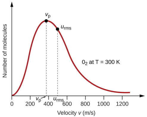
Most Probable speed/velocity
The y-axis of the graph represents the number of molecules. So, the taller the graph is, the more will be the number of molecules having similar energy. In fact, the point at the tip of the curve corresponds to the velocity at which most of the molecules are moving. In other words, most of the molecules have that velocity. Hence, if we randomly pick up a molecule, the chances of it having this velocity is more than having any other value of velocity. Hence, the datum at the top of the graph points to the most probable velocity. This also indicates that there are only very few particles that have a velocity that is lower than the most probable velocity. The same inference can be drawn for the particles with very high speeds.
Average speed
The top of the curve represents the most probable speed. It indicates that most of the molecules are moving at that speed. However, it is not the average speed. Average speed is actually represented by a position that would be present on the right side of the most probable speed. The reason for this lies in the fact that the average speed cannot be less than the speed that is possessed by most of the gaseous molecules. At the same time, it cannot be equal to that also, simply because the molecules at the far right of the curve possess extremely high speeds. It is to be noted that this property is a scalar quantity and there is no equivalent average velocity (which is zero) because the direction of particles under motion is random.
Root Mean Squared speed
Root mean squared speed basically means the square root of the average of the squares of the individual molecular speeds. For a statistical distribution like a bell curve (normal distribution), the statistical probability is better represented by the square of the values deviating from the most probable one. In the case of Boltzmann distribution, it is placed on the right side of average speed since the squares of the higher values would outweigh those with smaller values even though the numbers are less for the former. The RMS value is once again, as the average, a scalar quantity and hence represented as speed and not velocity.
An understanding of these three basic points on the curve helps us to extract the information that is summarized in a Boltzmann distribution curve.
Reading the Maxwell-Boltzmann Distribution curve
Individual points on the curve
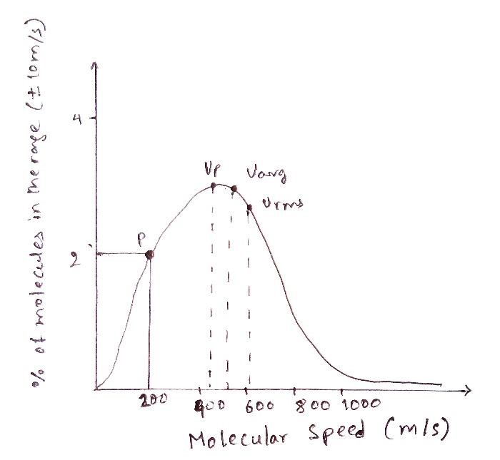
Let’s consider any point “p” on the graph. A quick recap of the terms on the x and the y-axes is beneficial at this stage. The number of molecules represented on the y-axis refers to the number of molecules within a certain speed range since, as we have seen, it is highly unlikely that the values would be exactly equal owing to the random motion.
A slight adjustment to the y-axis can be made by naming it as the “percentage of molecules” within the speed range of v+dv, where v is the speed (represented by the y-axis) and DV is the deviation in it. In other words, If we plot a graph to find out the percentage of molecules that have a velocity in the range of, say 10 m/s of the speed 200 m/s, then the point (x,y) where the perpendiculars from the axes meet, is the point “p”.
Let’s assume that the value of p comes out to be 2%. What it means is that if we randomly pick 1000 molecules from the gas, 20 out of those would have the velocity in the range of ±10 m/s of 200 m/s. However, it does not mean that all of these 20 or any of these 20 molecules have a velocity of exactly 200 m/s. The point “p” also does not indicate any fixed number, it indicates the percentage. As we may recall, the number of molecules between any two points is given by the area below the curve.
Extracting the useful information
Hot and cold systems
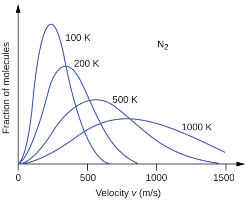
The importance of the Boltzmann distribution curve can be further emphasized by the information it holds about the temperature of the system. At higher temperatures, the kinetic energy of the molecules is higher. As a result, most of the molecules attain greater speeds. This is very well reflected in the flattening of the curve. With increasing temperature, the number of molecules having similar speeds reduces significantly. The top of the curve moves towards the right and the shape becomes broader.
The converse situation is observed under the effect of cooling. As a gas becomes cooler, the kinetic energy of the molecules decreases significantly and most of the molecules move at a slower speed. The effect can be distinctly seen in the distribution curve which becomes narrower along with the increase in its height and shift towards the left. The interesting feature that holds true for both hot and cold systems and anything intermediate in between is that the total area under the curve remains constant. This observation has to be consistent since the number of particles is not altered during heating or cooling. However, the number of gases that move towards higher energy is indeed more in the flattened curve.
Distribution according to molecular weights
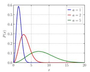
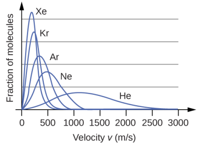
The Boltzmann distribution also holds information about the molecular mass of the gas. Taking into consideration the noble gases, if the distribution curve is plotted at the same temperature and pressure and includes the exact same moles of the gases, the outcome clearly displays that heavier gases tend to have more number of slowly moving molecules than the lighter ones. As a consequence, the curves increasingly become narrower and higher according to the increasing order of their molecular weights.
Summing up the importance of the Boltzmann Distribution – explanations for common observations
- The biggest achievement of Maxwell-Boltzmann distribution is the explanation that the regular macroscopic behaviour of the gases has an underlying random microscopic behaviour.
- Since the molecular mass of a gas is directly proportional to the speeds at which its molecules move, this observation can be related to the fact that hydrogen is likely to escape away from atmosphere at higher altitudes compare to oxygen and nitrogen. At the same time, carbon dioxide remains near the ground due to its higher molecular weight.
- The Boltzmann distribution is applicable to not only gases but even to solids and liquids. The most obvious display of this phenomenon is the evaporation of liquids below the boiling point. Although most of the molecules of a liquid are not as mobile as gas molecules, still some of these, residing on the surface, have more speeds than the ones in the bulk. These can escape to the surroundings. The rate of evaporation is accelerated upon increasing the temperature, which is aptly displayed by water, a common observation during summer times.
Frequently Asked Questions
What is Maxwell-Boltzmann distribution?
Maxwell-Boltzmann distribution is a probability distribution attributed to describe the velocities of different particles having different kinetic energies in a stationary container at a constant temperature.
What is the Maxwell-Boltzmann distribution curve?
The Maxwell-Boltzmann distribution curve plots the fraction of molecules on the y-axis and their velocities on the x-axis at a specific temperature. Since the speed of gas molecules is variable at any temperature, the curve is always smooth without sharp edges.
What is the effect of temperature on the Maxwell-Boltzman distribution curve?
An increase in temperature increases the number of molecules having greater velocities, so the curve gets broader and moves to the right. On the other hand, a decrease in temperature decreases the number of molecules, and most of the molecules have an average velocity, so the curve narrows down and moves to the left.
What is the importance of Maxwell-Boltzman distribution?
Maxwell-Boltzmann's distribution gave an idea that the typical macroscopic behaviour of gases has a random underlying behaviour of molecules. This idea of variable kinetic energies and velocities of molecules also applies to liquids and solids.
References
- Physical Chemistry, 9th Edition by Peter Atkins & Julio de Paula
- Chemistry 2e, an OpenStax resource
- https://homepage.univie.ac.at/franz.vesely/sp_english/sp/node8.html
- https://deepai.org/machine-learning-glossary-and-terms/maxwell-boltzmann-distribution
- Camuffo, D. Consequences Of The Maxwell–Boltzmann Distribution. Microclimate for Cultural Heritage 2019, 61-71.
If you like what you read and you're teaching or studying A-Level Biology, check out our other site! We also offer revision and teaching resources for Geography, Computer Science, and History.